

 trading
Mastering Options Portfolio P&L: A Comprehensive Guide to Delta-Gamma Approximation

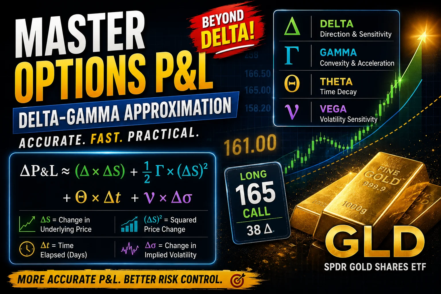
Understanding and accurately forecasting Profit and Loss (P&L) is essential for quantitative traders, portfolio managers, and options strategists. Although Delta-based estimation is widely used for quick calculations, relying exclusively on Delta can produce significant errors, particularly during periods of high volatility or substantial movements in the underlying asset price.
This guide explores the Delta-Gamma Approximation Method, demonstrating how incorporating second-order sensitivity (Gamma), alongside Theta and Vega, can improve options P&L estimates.
To illustrate its practical application, we will examine a hypothetical trading scenario involving options on GLD (SPDR Gold Shares ETF).
1. Introduction: Why First-Order Delta Is Not Enough
Most options traders use Delta ((\Delta)) as their primary measure of directional exposure.
Delta represents the rate of change in an option’s price relative to a change in the underlying asset’s spot price.
Mathematically:
Where:
- (V) = Option Price
- (S) = Underlying Spot Price

Advanced Options Trading in plain English | (Options Trading)
Course Specifications
- 18.5 Hours of HD Video Training: Full-length lessons in crisp 1080p resolution with English subtitles.
- Last Updated: February 2023
- File Size: 7.56 GB.
The Limitation of Linear Estimation
Delta-based estimation assumes that the option’s sensitivity to the underlying asset price remains constant over the price movement being analyzed.
However, this assumption is not entirely accurate.
Options exhibit non-linear price behavior, commonly referred to as convexity. As the underlying asset price changes, Delta itself changes.
This is precisely where Gamma becomes important.
- Positive Gamma (Long Options): Delta increases when the underlying price rises and decreases when the underlying price falls. This generally benefits long-option positions by creating favorable convexity.
- Negative Gamma (Short Options): Delta moves against the position as the underlying price changes, potentially accelerating losses during substantial market movements.
Ignoring Gamma can therefore lead to meaningful errors in estimated P&L, particularly when the underlying asset experiences large price movements.
2. The Mathematical Foundation: Taylor Series Expansion
To capture the non-linear relationship between an option’s price and its underlying variables, we can use a second-order Taylor Series approximation.
This approach incorporates four primary options Greeks:
- Delta ((\Delta)): First-order sensitivity to the underlying asset price.
- Gamma ((\Gamma)): Second-order sensitivity to the underlying asset price.
- Theta ((\Theta)): Sensitivity to the passage of time.
- Vega ((\mathcal{V})): Sensitivity to changes in implied volatility.
The Full P&L Approximation Equation
The estimated change in an option position’s value can be expressed as:
Where:
- (\Delta P&L) = Estimated change in position value.
- (\Delta S) = Change in the underlying asset price.
- ((\Delta S)^2) = Squared change in the underlying asset price.
- (\Delta t) = Time elapsed, expressed in the same time unit used for Theta.
- (\Delta \sigma) = Change in implied volatility.
- (\Delta) = Delta.
- (\Gamma) = Gamma.
- (\Theta) = Theta.
- (\mathcal{V}) = Vega.
Important: This is a truncated Taylor approximation. It assumes that the Greeks remain approximately constant over the modeled changes and excludes higher-order sensitivities and interaction effects, such as Vanna and Volga.
3. Case Study: Long Call Option on GLD ETF
To demonstrate the practical application of the Delta-Gamma approximation, consider a hypothetical market scenario involving GLD (SPDR Gold Shares ETF).
Initial Position Parameters
| Parameter | Value |
|---|---|
| Underlying Spot Price ((S)) | $161.00 |
| Option Position | Long 1 × 165 Call |
| Initial Delta | 0.3774 |
| Purchase Premium | $3.20 per share |
| Contract Multiplier | 100 |
| Total Initial Premium | $320.00 |
Position Greeks
The following Greeks are expressed at the contract level, rather than on a per-share basis.
| Greek | Contract-Level Value | Interpretation |
|---|---|---|
| Delta ((\Delta)) | +37.74 | P&L change per $1 underlying move |
| Gamma ((\Gamma)) | +3.36 | Change in Delta-equivalent exposure per $1 move |
| Theta ((\Theta)) | -$7.27 | Daily time decay |
| Vega ((\mathcal{V})) | +$17.70 | P&L change per 1 volatility percentage point |
These values are assumed inputs for the hypothetical example, not verified historical market quotes.
4. Market Shift Simulation: Step-by-Step P&L Calculation
Suppose overnight market developments trigger the following changes:
- Underlying Price Movement ((\Delta S)): +$10.00
- Time Elapsed ((\Delta t)): 1 Day
- Implied Volatility Change ((\Delta \sigma)): +10 percentage points
We can now calculate the estimated P&L contribution of each Greek.
Step 1: Delta Contribution
Delta measures the initial directional exposure of the option position.
Substituting the values:
Step 2: Gamma Contribution
Gamma captures the non-linear component of the option’s price movement.
The second-order Gamma contribution is calculated using:
Substituting the values:
Key Takeaway:
Gamma contributes an additional $168.00 to the estimated gain.
A trader relying exclusively on Delta would miss this second-order contribution, which represents approximately 30.8% of the combined Delta and Gamma profit.
This demonstrates why Gamma becomes increasingly important during substantial underlying price movements.
Step 3: Theta Contribution
Theta measures the impact of time decay on the option’s value.
For a long call position, Theta is generally negative, meaning the option loses value as time passes, all else being equal.
Substituting the values:
]
]
Step 4: Vega Contribution
Vega measures the sensitivity of an option’s price to changes in implied volatility.
Since the position has positive Vega, an increase in implied volatility generally increases the option’s value.
]
Assuming Vega is quoted per one percentage point of implied volatility:
]
]
Important: A 10-percentage-point increase means, for example, an increase in implied volatility from 25% to 35%, not from 25% to 27.5%.
Step 5: Total Estimated P&L
We can now combine all four contributions:
[
]
Therefore:
[
This represents the estimated profit after accounting for the initial $320 premium, assuming the option was purchased at that price and the position consists of one standard 100-share contract.
The estimated ending position value is:
[
$320.00+$715.13=$1,035.13
]
All calculations exclude commissions, transaction costs, and execution slippage.
5. Approximation vs. Exact Pricing Simulation
To evaluate the effectiveness of the Delta-Gamma approximation, we can compare the theoretical estimate against an independently calculated option-pricing simulation.
Consider the following illustrative results:
| Metric | Approximation Model | Pricing Simulation | Difference |
|---|---|---|---|
| Initial Position Value | $320.00 | $320.00 | $0.00 |
| Estimated Final P&L | +$715.13 | +$721.10 | $5.97 |
Accuracy Analysis
The absolute difference between the two estimates is:
|715.13-721.10|
The relative error compared with the simulated P&L is:
This corresponds to approximately 99.17% relative closeness between the two illustrative results.
However, this comparison should not be interpreted as proof that the approximation consistently achieves greater than 99% accuracy.
Actual accuracy depends on market conditions, the size of the underlying price movement, changes in implied volatility, time to expiration, and the higher-order Greeks omitted from the approximation.
The main advantage of the method is that it provides a fast and computationally efficient estimate without requiring a complete option repricing model for every scenario.
6. Practical Applications in Risk Management and After-Hours Hedging
The Delta-Gamma approximation has several practical applications in professional trading and portfolio risk management.
6.1. After-Hours Equity and Futures Hedging
Options markets may close while the underlying equities and futures markets continue trading.
During these periods, traders may need to estimate how their options exposure changes as the underlying asset moves.
The Delta-Gamma framework helps estimate the updated directional exposure:
This provides a useful approximation of the new Delta and helps risk managers estimate the underlying shares or futures contracts required for delta hedging.
However, the hedge must also account for contract multipliers, futures conversion factors, and other relevant portfolio exposures.
6.2. Managing Tail Risk in Short-Option Strategies
Short-call and short-put positions generally carry negative Gamma.
As the underlying asset moves, the position’s Delta can change unfavorably, causing losses to accelerate.
By incorporating Gamma into risk calculations, traders can better understand the non-linear behavior of short-option positions.
This can improve:
- Dynamic hedging decisions.
- Position sizing.
- Scenario analysis.
- Risk-limit calculations.
- Stop-loss and exposure management.
Gamma is particularly important when managing short-option strategies during earnings announcements, economic releases, and other periods of elevated market volatility.
7. Limitations and Best Practices
Although the Delta-Gamma approximation is a powerful analytical tool, it is not a substitute for a complete option-pricing model.
Its reliability depends on several assumptions:
- Greeks are calculated using the same underlying pricing and contract conventions.
- Changes in the underlying price and implied volatility are not excessively large.
- Theta and Vega are applied using their correct time and volatility units.
- Higher-order Greeks and interaction effects are sufficiently small.
- The volatility surface, interest rates, dividends, and other pricing inputs do not change in ways that materially affect the result.
For particularly large market movements, a full repricing of the option using an appropriate pricing model is preferable.
Essential Best Practices
1. Small Underlying Price Movements
For relatively small changes in the underlying asset price, Delta alone may provide a reasonable first-order estimate.
2. Large Underlying Price Movements
Gamma becomes increasingly important as the underlying asset moves further away from its initial price.
Ignoring the second-order term can lead to substantial estimation errors.
3. Significant Implied Volatility Changes
Vega must be incorporated whenever implied volatility changes materially, particularly for options with substantial volatility exposure.
4. Time Decay and Expiration
Theta becomes increasingly relevant as expiration approaches, although its behavior depends on the option’s moneyness and market conditions.
5. Full Repricing for Critical Risk Decisions
When precision is essential, use a full option-pricing model rather than relying exclusively on a truncated Taylor approximation.
8. Conclusion
The Delta-Gamma approximation provides a more comprehensive approach to options P&L estimation by incorporating both linear and non-linear price sensitivities.
By combining Delta, Gamma, Theta, and Vega, traders can develop a more informative estimate of how an options position responds to changes in the underlying asset price, the passage of time, and implied volatility.
The central principle is straightforward:
Delta explains the initial directional exposure, Gamma captures the curvature of the price response, Theta accounts for time decay, and Vega measures sensitivity to implied volatility.
For quick scenario analysis and preliminary risk assessment, the combined framework offers a practical alternative to Delta-only calculations.
Ultimately, understanding all four Greeks is essential for more informed options trading, dynamic hedging, and portfolio risk management.